About
OCT Overview
|
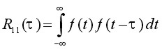
Introduction Optical Coherence Tomography (OCT) is an optical signal acquisition and processing method. Its purpose is to interpret interferometric data and transform it into a 2D or 3D image. A coherent beam of light is split into two separate beams, a reference arm and sample arm. The sample arm focuses into the tissue being observed, and the reference arm reflects back from a flat optical mirror. These two beams then interfere and cause either amplification or negation of the signal based upon the phase and time delay of the backscatter light from the sample. This amplification is detected and then translated into an image. In OCT, near-infrared light is often used because of its high penetration depth in samples such as tissue. This longer wavelength of light is less affected by the scattering coefficient of the sample (which is wavelength dependent), so the light can travel farther into the tissue before being completely scattered. OCT is a useful technique because it can create micrometer-resolution three-dimensional images of the sample. This is very valuable in the field of diagnostic medicine. OCT is based upon white light interferometry. Interference occurs between the light that is back scattered from the sample and light that has traveled a known distance in the reference arm. The incident light source is split into the reference beam, with electric field Er(t) and the sample arm with Es(t). These beams travel two different lengths in each arm, and the output of the interferometer is the sum of these two fields. The detector then measures the intensity, which is proportional to the square of the summed field: Io ~ |Er(t)| + |Es(t)| + 2ErEscos(2kDL) (1) Where DL is the path length difference of between the two arms. If the reference path length is scanned, then interference fringes will be generated as a function of time. In a system that uses a broad-bandwidth (or low-coherence) source such as in OCT, interference will only occur when the path lengths are matched to within the coherence length of the source around OPD = 0. This can be seen with simple white light fringes in a Michelson interferometer, that only occur very close to OPD = 0. The coherence length is inversely proportional to the bandwidth of the source, which also controls the resolution of the system. In OCT, the interferometer measures the magnitude and field autocorrelation of the light. The equation for field autocorrelation is:
Autocorrelation gives an indication as to what degree the time signal is displaced. This allows us to determine the echo time of the signal, which then translates to depth in the tissue. The echo time and magnitude are translated into an electrical signal called an A-scan. Each scan through the tissue is translated into an axial scan or an A-scan. The A-scan is the electric signal that results from levels of high and low amplification caused by interference in the sample along with echo time delay, or the delay in the signal because of depth in the tissue.
Each A-scan is one pulse of the reference mirror. If the sample isn’t moved, then the same A-scan will be taken over and over in the same place. To create a two-dimensional image, the sample is either moved while the A-scans are being taken, or a part of the sample arm will translate to focus the light onto different parts of the sample. This is done so that thousands of A-scans are taken over a lateral range of the tissue, which creates a 2D image. To create a 3D dimensional image, the A-scans are taken in a raster pattern over the sample. Setup:
The optical setup of OCT is very similar to the setup of a Michelson Interferometer. However, in a Michelson
Interferometer, both arms of the device contain flat mirrors. In OCT one of the arms contains a sample, which
will scatter light, just not as uniformly as a mirror. The second (reference) mirror also fluctuates, as
described before, to allow the OPD to be equal to zero at different depths in the tissue. The recombined beam
of light is sampled by a detector that translates the intensity of the light into an electrical signal.
Figure 2. Diagram of OCT Setup which demonstrates its similarity to a Michelson Interferometer [2]
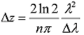
Expected Outcome Standard Images created by OCT have micrometer-resolution that highlights inhomogeneous areas in the sample. The images we produce should have similar results. The changes in the sample cause changes in refractive index as well as physical reflecting surfaces. These show up as lighter areas in images, where as the areas of low scattering and reflection appear as dark areas in the tissue. The standard axial resolution of OCT is between 4 and 10 microns. Both images from other sources and images taken by the authors will be displayed in the results section. Measurements The images that are produced are a result of the digital signal created by the OCT setup. A-scans are combined into an image that demonstrated areas of tissue change in the sample. To take images, most OCT systems use light sources with a center bandwidth between 800-1300 nanometers. As stated before, this is due to the fact that infrared light has greater penetration depth and reduced scattering compared to visible and UV. Also, no light with a wavelength longer than 1300 nanometers is used because water absorbs light beyond this region. Most tissue is made mostly of water, so the tissue simply absorbs the light instead of scattering it. Most sources have a bandwidth of about 100 nm, which provides and axial resolution between 4 – 10 microns. This can be seen in the equation for axial resolution:
Dz is the axial resolution, Dl is the bandwidth, and l is the central wavelength. From this is it is clear that a broader
bandwidth would leader to a smaller axial resolution. However, only specialized sources can attain extremely wide bandwidth,
so the standard is around 100 nm.
Data and Results:
The bottom three images demonstrate a resolution of 5 microns axial resolution and 10 microns lateral resolution. Conclusion OCT is a very useful technique for visualizing scattering materials at high resolution. This makes it very useful in the field of diagnostic medicine. OCT has come to be called the “optical biopsy” for this very reason. It can be used to visualize tissue below the surface without having to remove the tissue from the body, which has obvious benefits over a biopsy. It is currently most commonly used in ophthalmology for taking high resolution, non-invasive images of the retina, something that cannot easily be done with any other technique. This is very useful because biopsies of the eye cannot be taken without causing permanent blindness, so it is often very hard to diagnose retinal ailments without OCT. It is also used for the diagnosis of coronary artery disease, because OCT is able to identify plaque build up on the inside of arteries. Some types of OCT can even visualize the blood flow inside the artery, which can be helpful in diagnosing different types of heart disease. OCT is also used for monitoring patients who have a high risk of getting cancer. Because OCT can take such high-resolution images, it is possible to see very small changes in tissue that are often indicative of cancer development. This allows for very early detection of cancer in a way that does not require biopsy, which is the current medical standard. References 1. Krijen, Kees. “Autocorrelation.” Particle Sizing related Static, Dynamic and Electrophoretic LLS Instrumental Experiments. 1999. <sfprime.net/lls/index.htm> 2. Drexler, Wolfgang and James Fujimoto. Optical Coherence Tomography: Technology and Applications. Berlin: Springer, 2008. Images The authors took all images not cited. [1] Winkler, Amy. A-scan. Tissue Optics Lab. Tucson, AZ. [2] Pumpkinegan, OCT B-Scan Setup. < http://en.wikipedia.org/wiki/File:OCT_B-Scan_Setup.GIF> [3] Browning DJ, Fraser CM, Clark S. The relationship of macular thickness to clinically graded diabetic retinopathy severity in eyes without clinically detected diabetic macular edema. Ophthalmology2008;115:533-9 |
 (2)
(2)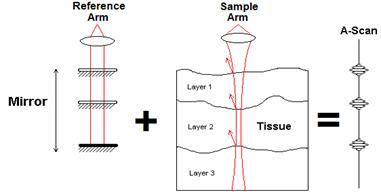 Fig 1. Visual Representation of an A-scan [1]
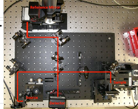 Fig 2.2 . Picture of an OCT setup with the light path drawn in.
This electrical signal is translated by the image processing programs written for the device
used. The image is then displayed on the computer running the control program.
Fig 2.2 . Picture of an OCT setup with the light path drawn in.
This electrical signal is translated by the image processing programs written for the device
used. The image is then displayed on the computer running the control program.
 (3)
(3)
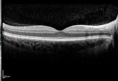 Fig 3. OCT scan of a retina showing a thickened retina associated with diabetic macular oedema. The central dip is caused
by the retinal nerve, and the different layers can be visualized. [3]
Fig 3. OCT scan of a retina showing a thickened retina associated with diabetic macular oedema. The central dip is caused
by the retinal nerve, and the different layers can be visualized. [3]
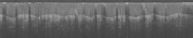
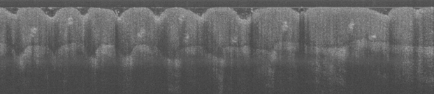 Fig 4. Two OCT images of the thumb tip taken by the authors in the Tissue Optics Lab. Features such as the epidermis,
fingerprints, and sweat glands can be seen.
Fig 4. Two OCT images of the thumb tip taken by the authors in the Tissue Optics Lab. Features such as the epidermis,
fingerprints, and sweat glands can be seen.
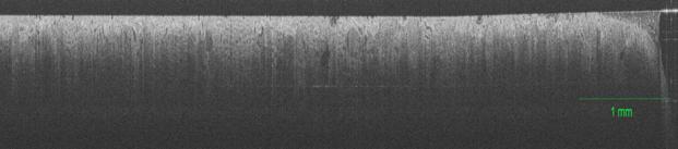 Fig 5. OCT image of a healthy kidney where features such as blood vessels and glomeruli can be seen.