|
To convert our time domain OCT system into a spectral
domain OCT system, the photodiode detector is replaced with a CCD-based
spectrometer. The specifications for the spectrometer are dictated by the
light source spectrum, the depth resolution, and the imaging depth.
The depth resolution should ultimately be limited by the light source,
via the coherence length:
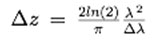 where Δz and Δλ are the full widths at half maximum (FWHM) for the depth point
spread function and the source bandwidth respectively assuming a Gaussian
source spectrum.
Ideally, the imaging depth should be limited by the scattering properties of
the sample at the source wavelengths. For most applications in our lab, we
are limited due to scattering at 1-2 mm.
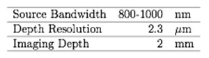
Considering this parameters for our light source, which emits light from
800-1000 nm, the spectrometer specifications are given in the following
table.
where Δz and Δλ are the full widths at half maximum (FWHM) for the depth point
spread function and the source bandwidth respectively assuming a Gaussian
source spectrum.
Ideally, the imaging depth should be limited by the scattering properties of
the sample at the source wavelengths. For most applications in our lab, we
are limited due to scattering at 1-2 mm.
Considering this parameters for our light source, which emits light from
800-1000 nm, the spectrometer specifications are given in the following
table.
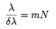
 In spectral domain OCT, like time domain OCT, the depth resolution of the
system depends on the detected spectral bandwidth. For this CCD-based
spectrometer design, the entire spectral bandwidth, from 800-1000 nm must
be imaged onto the pixel array.
The imaging depth, zmax, is related to the spectral resolution, δλ, in the
same way that the spectral bandwidth, Δλ, is related to the depth resolution,
Δz. Both are linked via the Fourier Transform, so
In spectral domain OCT, like time domain OCT, the depth resolution of the
system depends on the detected spectral bandwidth. For this CCD-based
spectrometer design, the entire spectral bandwidth, from 800-1000 nm must
be imaged onto the pixel array.
The imaging depth, zmax, is related to the spectral resolution, δλ, in the
same way that the spectral bandwidth, Δλ, is related to the depth resolution,
Δz. Both are linked via the Fourier Transform, so
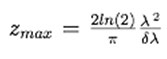 Therefore, δλ should be no greater than:
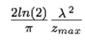 The greatest restriction on δλ occurs at the minimum wavelength, λ = 800 nm,
or δλ ≤ 0.14 nm.
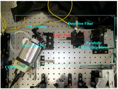
The spectrometer design contains four main components: a collimator, a
spectrally dispersive element, a focusing lens, and a detector array. In
the design of this spectrometer, the constrains begin at the detector,
which is the most expensive element, the choice of which subsequently
constrains the other components.
The greatest restriction on δλ occurs at the minimum wavelength, λ = 800 nm,
or δλ ≤ 0.14 nm.
The spectrometer design contains four main components: a collimator, a
spectrally dispersive element, a focusing lens, and a detector array. In
the design of this spectrometer, the constrains begin at the detector,
which is the most expensive element, the choice of which subsequently
constrains the other components.
 CCD Array
To achieve a spectral resolution of δλ ≤ 0.14 nm and detect the full 200 nm bandwidth, a minimum of 200 / 0.14 ≈ 1,429 pixels is required. Commercially available CCD arrays typically come with a number of pixels factorable by two (512, 1024, 2048, 4096).
At the time this spectrometer was designed, CCD arrays with up to 4096 pixels were commercially available. The specifications of these arrays showed that pixel arrays with 2048 pixels had larger pixel sizes than arrays with 4096 pixels, resulting in less read-out noise. Larger pixel size also loosens the geometric spot size specification for the focusing optic. Therefore, a CCD array with 2048 pixels was chosen.
The commercial CCD array selected is an Atmel Aviiva M2 CL Linescan Camera (San Jose, CA) with 2048 pixels and a 14 μm pitch. Each pixel is 14 μm by 14 μm with no spacing between pixels resulting in a 28.672 mm array length.
Grating
Spectral dispersion can be accomplished with a prism or a grating. Gratings are typically used because high spectral resolution can be achieved with a relatively small beam diameter and also because they are less bulky.
The spectral resolution of a grating, δλ, is limited by the diffraction order, m, and the number of periodic grooves illuminated, N, as shown:
CCD Array
To achieve a spectral resolution of δλ ≤ 0.14 nm and detect the full 200 nm bandwidth, a minimum of 200 / 0.14 ≈ 1,429 pixels is required. Commercially available CCD arrays typically come with a number of pixels factorable by two (512, 1024, 2048, 4096).
At the time this spectrometer was designed, CCD arrays with up to 4096 pixels were commercially available. The specifications of these arrays showed that pixel arrays with 2048 pixels had larger pixel sizes than arrays with 4096 pixels, resulting in less read-out noise. Larger pixel size also loosens the geometric spot size specification for the focusing optic. Therefore, a CCD array with 2048 pixels was chosen.
The commercial CCD array selected is an Atmel Aviiva M2 CL Linescan Camera (San Jose, CA) with 2048 pixels and a 14 μm pitch. Each pixel is 14 μm by 14 μm with no spacing between pixels resulting in a 28.672 mm array length.
Grating
Spectral dispersion can be accomplished with a prism or a grating. Gratings are typically used because high spectral resolution can be achieved with a relatively small beam diameter and also because they are less bulky.
The spectral resolution of a grating, δλ, is limited by the diffraction order, m, and the number of periodic grooves illuminated, N, as shown:
 Most gratings are first order gratings, that is they are efficient at m = 1. The number of grooves illuminated, N, depends upon the density of the grooves as well as the beam diameter. Groove densities range from 200 grooves per mm up to 3600 grooves per mm. Groove densities between 200 and 1200 mm-1 are easily manufactured, and therefore relatively inexpensive.
To achieve δλ ≤ 0.14 nm, assuming m = 1, the number of illuminated grooves, N, must be at least 7,143. For a groove density of 1200 mm-1, the beam diameter must be 6 mm. This diameter is assuming uniform light distribution; however, this OCT system is fiber-based to facilitate endoscopic imaging, and light propagating in a single mode fiber has a Gaussian profile. Gaussian profiles are preferred for many applications because they retain their profile shape when propagated through space or through lenses, so long as the Gaussian beam is not clipped by an aperture. Beam clipping results in undesirable sidelobes, that limit system sensitivity. Diffraction from a Gaussian beam can be roughly equated to diffraction from a uniform beam by using the FWHM, ΔxFWHM in place of the uniform beam diameter. Therefore, the constraint for a Gaussian beam is that the FWHM is 6 mm, but the actual aperture size should be greater to minimize beam clipping. The FWHM is the diameter of the beam where the amplitude has dropped to 1/2 of the maximum. The beam diameter at 1/ϵ of the maximum can be found by the following equation:
Most gratings are first order gratings, that is they are efficient at m = 1. The number of grooves illuminated, N, depends upon the density of the grooves as well as the beam diameter. Groove densities range from 200 grooves per mm up to 3600 grooves per mm. Groove densities between 200 and 1200 mm-1 are easily manufactured, and therefore relatively inexpensive.
To achieve δλ ≤ 0.14 nm, assuming m = 1, the number of illuminated grooves, N, must be at least 7,143. For a groove density of 1200 mm-1, the beam diameter must be 6 mm. This diameter is assuming uniform light distribution; however, this OCT system is fiber-based to facilitate endoscopic imaging, and light propagating in a single mode fiber has a Gaussian profile. Gaussian profiles are preferred for many applications because they retain their profile shape when propagated through space or through lenses, so long as the Gaussian beam is not clipped by an aperture. Beam clipping results in undesirable sidelobes, that limit system sensitivity. Diffraction from a Gaussian beam can be roughly equated to diffraction from a uniform beam by using the FWHM, ΔxFWHM in place of the uniform beam diameter. Therefore, the constraint for a Gaussian beam is that the FWHM is 6 mm, but the actual aperture size should be greater to minimize beam clipping. The FWHM is the diameter of the beam where the amplitude has dropped to 1/2 of the maximum. The beam diameter at 1/ϵ of the maximum can be found by the following equation:
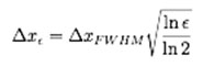 To collect out to 1% of the maximum (ϵ = 100), the aperture must be at least 15.5 mm in diameter, enabling the use of widely available one inch (clear aperture 22 mm typical) optical components.
The angular dispersion of the grating is determined by the grating equation,
To collect out to 1% of the maximum (ϵ = 100), the aperture must be at least 15.5 mm in diameter, enabling the use of widely available one inch (clear aperture 22 mm typical) optical components.
The angular dispersion of the grating is determined by the grating equation,
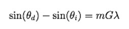 where θd is the dispersion angle referenced to the optical axis, θi is the angle of incidence, G is the groove density, and m is the grating order.
This equation is valid for a thin grating, but when the grating becomes thick, the efficiency for higher orders (m ≠ 1) and for wavelengths other than the design wavelength diminishes. For a limited wavelength and angular range, the efficiency can be quite high. The information about the wavelength / angular range is given by the grating manufacturer as the Bragg wavelength. When the grating meets the Bragg condition at the specified wavelength (dubbed the Bragg wavelength), efficiency above 80% is easily achieved.
Wasatch Photonics (Logan, UT) designs transmissive, holographic gratings near the wavelength range of our system, λBragg = 830 nm, with 1200 G/mm (1.2 G/μm). Typically, the manufacturer assumes an angle of incidence for which satisfies the grating equation when θd = -θi (although it is a good idea to check with the manufacturer on this point). At this wavelength, this angle of incidence is
where θd is the dispersion angle referenced to the optical axis, θi is the angle of incidence, G is the groove density, and m is the grating order.
This equation is valid for a thin grating, but when the grating becomes thick, the efficiency for higher orders (m ≠ 1) and for wavelengths other than the design wavelength diminishes. For a limited wavelength and angular range, the efficiency can be quite high. The information about the wavelength / angular range is given by the grating manufacturer as the Bragg wavelength. When the grating meets the Bragg condition at the specified wavelength (dubbed the Bragg wavelength), efficiency above 80% is easily achieved.
Wasatch Photonics (Logan, UT) designs transmissive, holographic gratings near the wavelength range of our system, λBragg = 830 nm, with 1200 G/mm (1.2 G/μm). Typically, the manufacturer assumes an angle of incidence for which satisfies the grating equation when θd = -θi (although it is a good idea to check with the manufacturer on this point). At this wavelength, this angle of incidence is
 When used away from this specific angle of incidence, high efficiency performance can be shifted to a different wavelength. The angle/wavelength pair to achieve high efficiency can be found using the Bragg condition,
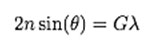
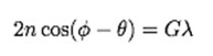 where n is the refractive index, λ is the wavelength, and G is the groove density. The angle θ refers to the angle of the incident beam, θi, inside the medium. This is not the same θi as described before which is in air. The angle ϕ refers to the slant of the grating grooves. For transmissive gratings that use the condition θd = -θi, ϕ is 90 degrees, meaning the grating grooves are parallel with the surface normal. Since ϕ is 90 degrees, the Bragg condition can be simplified to
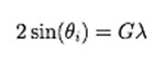
 Furthermore, Snell’s Law can be used to replace the incident angle in the medium θ with the incident angle in air, θi,
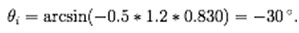
 The optimal efficiency for center wavelength λ = 900 nm occurs at θi = -33 degrees. The maximum efficiency in the specifications for this grating, provided by Wasatch Photonics, is 85%, which drops to about 60% at +/- 100 nm, in other words for 800 nm and 1000 nm.
Using θi = -33 degrees, the angular dispersion for 800-1000 nm can be determined using the grating equation. The spectrum from 800-1000 nm disperses approximately around 33 degrees +/- 8.1 degrees.
Collimator
Recall that to achieve the appropriate spectral resolution, the beam diameter of 15.5 mm at the 1% maximum is required. This beam diameter is determined by the focal length of the collimator and the numerical aperture (NA) of the fiber. The fiber in this spectrometer is Corning HI780, which has an NA of 0.14 at the 1% maximum. The NA is related to the angle, U, at which the light exits the fiber, as measured in the far field, into a material of refractive index n, as shown:
The optimal efficiency for center wavelength λ = 900 nm occurs at θi = -33 degrees. The maximum efficiency in the specifications for this grating, provided by Wasatch Photonics, is 85%, which drops to about 60% at +/- 100 nm, in other words for 800 nm and 1000 nm.
Using θi = -33 degrees, the angular dispersion for 800-1000 nm can be determined using the grating equation. The spectrum from 800-1000 nm disperses approximately around 33 degrees +/- 8.1 degrees.
Collimator
Recall that to achieve the appropriate spectral resolution, the beam diameter of 15.5 mm at the 1% maximum is required. This beam diameter is determined by the focal length of the collimator and the numerical aperture (NA) of the fiber. The fiber in this spectrometer is Corning HI780, which has an NA of 0.14 at the 1% maximum. The NA is related to the angle, U, at which the light exits the fiber, as measured in the far field, into a material of refractive index n, as shown:
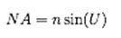 In this system, the fiber exits into air, so n = 1. The angle, U, for NA = 0.14 is approximately 8 degrees. The beam reaches 15.5 mm at:
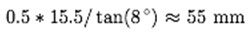 Therefore, the focal length of the collimator must be near 55 mm.
To collimate the beam with theoretically no aberrations, an off-axis, parabolic mirror is used. A number of off-axis, parabolic mirrors are available from Edmund Optics (Barrington, NJ). A parabolic mirror 30 degrees off-axis is used because in this configuration the fiber and fiber mount do not block the reflected light. The effective focal length (EFL) of the mirrors, as defined on the Edmund Optics website, is the distance from the focal point to the center of the mirror. The nearest available EFL to the calculated value of 55 mm is EFL=54.45 mm (Edmund Optics part number NT47-085).
Focusing Optic
The focusing optic focuses the spectrally dispersed light from the grating onto the CCD array. The spectral range 800-1000 nm, dispersed at 33 degrees +/- 8.1 degrees, needs to be imaged onto the 28.672 mm array. The angular spread, Δθ = 2 * 8.1 degrees, and the length of the image plane, L = 28.672 mm determine the focal length of the optic,
Therefore, the focal length of the collimator must be near 55 mm.
To collimate the beam with theoretically no aberrations, an off-axis, parabolic mirror is used. A number of off-axis, parabolic mirrors are available from Edmund Optics (Barrington, NJ). A parabolic mirror 30 degrees off-axis is used because in this configuration the fiber and fiber mount do not block the reflected light. The effective focal length (EFL) of the mirrors, as defined on the Edmund Optics website, is the distance from the focal point to the center of the mirror. The nearest available EFL to the calculated value of 55 mm is EFL=54.45 mm (Edmund Optics part number NT47-085).
Focusing Optic
The focusing optic focuses the spectrally dispersed light from the grating onto the CCD array. The spectral range 800-1000 nm, dispersed at 33 degrees +/- 8.1 degrees, needs to be imaged onto the 28.672 mm array. The angular spread, Δθ = 2 * 8.1 degrees, and the length of the image plane, L = 28.672 mm determine the focal length of the optic,
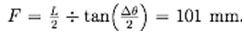 With 2048 pixels, the spectral resolution is smaller than necessary to achieve the specified image depth, so the 200 nm bandwidth may be imaged onto a subset of these pixels and still meet the image depth specification. This flexibility allows the focal length to be varied in the focusing optic design, allowing a lens design package to find an optimum solution (small spot size). Using this flexibility, the target system focal length is F ≈ 100 mm and allowed to vary during optimization.
The focusing optic design is a Cooke triplet, which uses multiple lenses to minimize all five third order Seidel aberrations (spherical, coma, astigmatism, field curvature, distortion). By choosing appropriate glass types, crown glasses for the outer, positive focal length elements and a flint glass for the central, negative focal length element, chromatic aberration can also be minimized. These aberrations can also be well-corrected over the specified field of view using a single lens with aspheric surfaces, but such custom optics can be expensive. Using multiple lenses allows for greater flexibility when trying to match commercially available lenses to decrease the cost of the optic.
The starting point for this lens is taken from Kingslake's book, Lens Design Fundamentals. A Cooke triplet lens is described in the book for photography, using the visible bandwidth, 400-700 nm, a focal length of 10 units (f-number, f/4.5), and a field of view of +/-20 degrees. Using this starting point, a lens design software package, such as Zemax, can optimize a new solution for the appropriate bandwidth (800-1000 nm), focal length (100 mm), and field of view (+/-8.1 degrees). After inputting the values for the surface curvatures, spacings, and refractive indices given in Kingslake (page 293), I scaled the f/4.5 system to have a focal length of 109 mm. Then, I incrementally optimized using standard glasses (BK7 and SF11), the appropriate bandwidth (800-1000 nm), and lower field of view (+/-8.1 degrees). I limited the lens apertures to 22 mm, consistent with commercially available optics. I also incrementally moved the system stop from the center of the system to outside of the system, since the physical system stop in this design is the diffraction grating. After incrementally optimizing for the appropriate system parameters, I began searching for commercially available lenses to fit the curvatures defined by Zemax. I split the middle lens, so that I could use two different lenses to better match the defined curvatures. I optimized the remaining optics after finding each commercially available match.
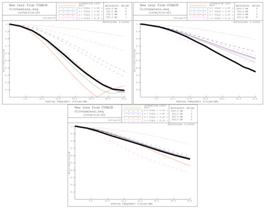
The metric used to optimize the lens design is the Modulation Transfer Function (MTF). The MTF assesses the ability of the optic to capture spatial frequencies. The y-axis is the visibility of the spatial frequency in the image plane, and the x-axis is the spatial frequency. Ultimately, the CCD array should limit the maximum spatial frequency, dictated by the pixel size. A pixel array with 14 μm pixels samples at spatial frequency, fsampling = 1 / 0.014 = 71.4 mm-1. As described by the Nyquist sampling theorem, the maximum recovered frequency is half the sampling frequency, fmax = fsampling / 2 = 35.7 mm-1. Therefore, the MTF from 0 to 35.7 mm-1 is the optimization metric.
On a side note, the design was started in Zemax and finished in Code V due to the availability of software packages. Either lens design package, in general, is capable of the full design. The figures shown are from Code V.
The final design is shown below. The lens vendors, part numbers, curvatures, and spacings are given in the table immediately following. The table is formatted as in Zemax and Code V, where each row corresponds to a surface. The surface has a radius of curvature and a protruding distance following it (center or edge thickness). The space following the surface is filled with either glass (specified) or air (default). Lenses are labeled at the first surface.
With 2048 pixels, the spectral resolution is smaller than necessary to achieve the specified image depth, so the 200 nm bandwidth may be imaged onto a subset of these pixels and still meet the image depth specification. This flexibility allows the focal length to be varied in the focusing optic design, allowing a lens design package to find an optimum solution (small spot size). Using this flexibility, the target system focal length is F ≈ 100 mm and allowed to vary during optimization.
The focusing optic design is a Cooke triplet, which uses multiple lenses to minimize all five third order Seidel aberrations (spherical, coma, astigmatism, field curvature, distortion). By choosing appropriate glass types, crown glasses for the outer, positive focal length elements and a flint glass for the central, negative focal length element, chromatic aberration can also be minimized. These aberrations can also be well-corrected over the specified field of view using a single lens with aspheric surfaces, but such custom optics can be expensive. Using multiple lenses allows for greater flexibility when trying to match commercially available lenses to decrease the cost of the optic.
The starting point for this lens is taken from Kingslake's book, Lens Design Fundamentals. A Cooke triplet lens is described in the book for photography, using the visible bandwidth, 400-700 nm, a focal length of 10 units (f-number, f/4.5), and a field of view of +/-20 degrees. Using this starting point, a lens design software package, such as Zemax, can optimize a new solution for the appropriate bandwidth (800-1000 nm), focal length (100 mm), and field of view (+/-8.1 degrees). After inputting the values for the surface curvatures, spacings, and refractive indices given in Kingslake (page 293), I scaled the f/4.5 system to have a focal length of 109 mm. Then, I incrementally optimized using standard glasses (BK7 and SF11), the appropriate bandwidth (800-1000 nm), and lower field of view (+/-8.1 degrees). I limited the lens apertures to 22 mm, consistent with commercially available optics. I also incrementally moved the system stop from the center of the system to outside of the system, since the physical system stop in this design is the diffraction grating. After incrementally optimizing for the appropriate system parameters, I began searching for commercially available lenses to fit the curvatures defined by Zemax. I split the middle lens, so that I could use two different lenses to better match the defined curvatures. I optimized the remaining optics after finding each commercially available match.
The metric used to optimize the lens design is the Modulation Transfer Function (MTF). The MTF assesses the ability of the optic to capture spatial frequencies. The y-axis is the visibility of the spatial frequency in the image plane, and the x-axis is the spatial frequency. Ultimately, the CCD array should limit the maximum spatial frequency, dictated by the pixel size. A pixel array with 14 μm pixels samples at spatial frequency, fsampling = 1 / 0.014 = 71.4 mm-1. As described by the Nyquist sampling theorem, the maximum recovered frequency is half the sampling frequency, fmax = fsampling / 2 = 35.7 mm-1. Therefore, the MTF from 0 to 35.7 mm-1 is the optimization metric.
On a side note, the design was started in Zemax and finished in Code V due to the availability of software packages. Either lens design package, in general, is capable of the full design. The figures shown are from Code V.
The final design is shown below. The lens vendors, part numbers, curvatures, and spacings are given in the table immediately following. The table is formatted as in Zemax and Code V, where each row corresponds to a surface. The surface has a radius of curvature and a protruding distance following it (center or edge thickness). The space following the surface is filled with either glass (specified) or air (default). Lenses are labeled at the first surface.
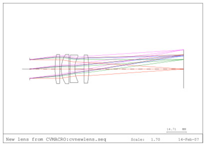
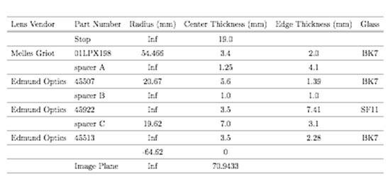 The spacers are custom machined aluminum rings with an outer diameter of 25 mm and inner diameter of 23 mm. The thickness of the rings is equivalent to the edge thickness given in the table. Varying the lens spacings in Code V shows that errors in lens spacing of+/- 0.05 mm minimally influence the Modulation Transfer Function (MTF) out to 35.7 mm-1. This precision is easily achieved. The lenses and spacers are mounted in a C-mount extension tube from Edmund Optics (part number NT58-736).
The following figure shows the MTF for 800, 900, and 1000 nm. The MTFs are shown separately for different wavelengths because the wavelengths are spatially separated by the grating and do not superimpose. The contrast drops to 0.1, 0.4, and 0.5 at 35.7 mm-1 for 800, 900, and 1000 nm respectively.
The spacers are custom machined aluminum rings with an outer diameter of 25 mm and inner diameter of 23 mm. The thickness of the rings is equivalent to the edge thickness given in the table. Varying the lens spacings in Code V shows that errors in lens spacing of+/- 0.05 mm minimally influence the Modulation Transfer Function (MTF) out to 35.7 mm-1. This precision is easily achieved. The lenses and spacers are mounted in a C-mount extension tube from Edmund Optics (part number NT58-736).
The following figure shows the MTF for 800, 900, and 1000 nm. The MTFs are shown separately for different wavelengths because the wavelengths are spatially separated by the grating and do not superimpose. The contrast drops to 0.1, 0.4, and 0.5 at 35.7 mm-1 for 800, 900, and 1000 nm respectively.
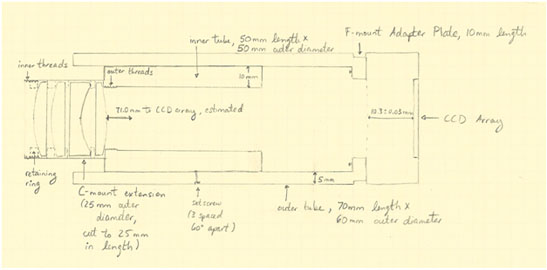
 The focusing optic is mounted in a C-mount extension tube, which is mounted to the CCD array camera using a standard F-mount adapter plate (Atmel) and custom aluminum tubes. The first tube is threaded to allow the C-mount extension to be attached. This tube fits into an outer tube. The outer tube contains through-holes at the back in order to attach with screws to the F-mount adapter plate. The tubes slip together to vary the length from the C-mount extension tube (containing the focusing optic) and the CCD array. The target distance from the final lens in the focusing optic to the CCD array is 71 mm. The tube length is set by three padded screws around the outside of the outer tube, locking the inner tube in place. This mount is illustrated in the following figure.
|